If you’re reading this, I know you probably know lots of ML algorithms, or perhaps used quite a few of them, say Logistic Regression, Decision tree, Stochastic boost, Random Forest, Lightgbm, Catboost (my favourite) and so on. I made one up, I guess you didn’t even notice. They’re just too many of them.

After data preparation, training a model is a key step in a machine learning pipeline, One needs to check the performance of the model irrespective of the algorithm used. You want to know if your model is actually learning from or just memorizing the data, this is where evaluation metrics play a vital role…

The choice of evaluation metric completely depends on the machine learning task. Say classification, regression, ranking, clustering, topic modelling, etc. For this article, we’ll be discussing common classification metrics. So grab a coffee and get ready to learn many new concepts and acronyms!

It’s important to note that for a classification task, its either we are predicting distinct classes (0/1) or probability estimates. We’ll be considering both cases.

Accuracy

A very simple and common classification metric is Accuracy

Classification accuracy is the ratio of correct predictions to total predictions made, say I got 45 questions correctly out of a total of 100 questions, accuracy would be 0.45 (45%)

Classification accuracy can also easily be turned into a misclassification rate or error rate by inverting the value i.e :

Simple right?.

It turns out most times, accuracy isn’t the best metric to use, imagine this scenario, As a machine learning engineer, your boss at work assigns you a task of building an ML model that accurately spot fraudulent transactions (a fraud detector), given customers transaction data where the target is to be 1 if the transaction is fraudulent or 0 if otherwise, You decide to use your favourite classifier, train it on part of the data, and test on a validation set, note that the validation set contains 9800 non-fraudulent transactions(i.e 0’s) and 200 fraudulent transactions (i.e 1's). andVoila, you get an accuracy of 97.5 % !!!. Badass right?

Well, before you get too excited, let’s look at a very dumb classifier that just classifies every single transaction to be a 0 i.e not fraudulent: if 0 is always predicted, then the classifier will be correct 9800 times and wrong 200 times, therefore:

A dumb classifier has an accuracy of 98% and yours has an accuracy of 97.5%. Still excited??.

This demonstrates why accuracy is generally not the preferred performance measure for classifiers, especially when you are dealing with skewed/imbalanced datasets (i.e., when some classes are much more frequent than others).

This brings us to Recall, Precision and F1 score, which are all derived from a table called Confusion matrix.

Confusion Matrix, Precision, Recall and F1-score

A much better way to evaluate the performance of a classifier is to look at the confusion matrix. The general idea is to count the number of times instances of class A are classified as class B and vice versa. In better terms, it tells us the types of incorrect predictions made by a classifier.

To compute the confusion matrix, you first need to have a set of predictions, so they can be compared to the actual targets.

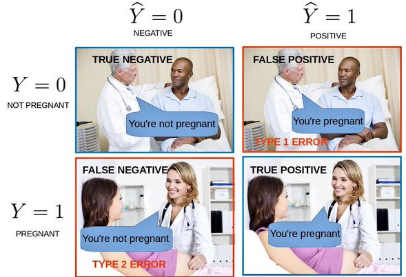
The confusion matrix itself is relatively simple to understand, but the related terminology can be confusing (the name itself, starting with ‘confusion’ isn’t helping matters). If you are confused about the confusion matrix (no pun intended), Figure 1.2 may help. This image would help you understand the terms.

Y represents the actual class(the truth) while Ŷ is the predicted class

figure 1.2

Lets properly define the terms we will be using.

• true positives (TP): These are cases in which we predicted yes (patient is pregnant), and she was truly pregnant
• true negatives (TN): We predicted no (not pregnant), and the patient wasn’t actually pregnant.
• false positives (FP): We predicted yes (pregnant), but the patient wasn’t pregnant. (Also known as a “Type I error.”)
• false negatives (FN): We predicted no (not pregnant), but the patient was actually pregnant (Also known as a “Type II error.”)

You can use the same explanation for the fraud detection scenario

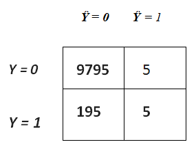
Now let’s assume that we got the below confusion matrix from our model’s prediction on the fraud detection dataset. The model was only able to detect 5 fraudulent cases out of 200 !! (i.e 195 false negatives FN’s). Imagine the amount of money customers will loose just because of your bad machine learning model.

TN = 9795

FN = 195,

FP = 5,

TP = 5

Recall (aka sensitivity):

This metric measures the ability of a model to find all the relevant cases within a dataset. The precise definition of recall is the number of true positives (TP) divided by the sum of true positives (TP) and false negatives (FN). In a more simple term, it answers the question — What proportion of actual positives was identified correctly? i.e When it’s actually yes, how often does it predict yes?. Therefore from the confusion matrix above recall is:

Actual Yes = Sum of the second row

Our model has a recall value of 0.025 — in other words, it correctly identifies only 2.5% of all fraudulent cases. terrible right?

Note: Recall is also called True Positive Rate (TPR)

Precision:

Unlike Recall, Precision attempts to answer the following question, What proportion of positive identifications was actually correct i.e When it predicts yes, how often is it correct?. The precise definition of precision is the number of true positives (TP) divided by the sum of true positives (TP) and false positives (FP). Therefore from the confusion matrix above precision is:

Predicted Yes = Sum of the second column

Our model has a precision value of 0.5 — in other words, when it predicts a fraudulent case, it’s correct 50% of the time.

F1- score:

The F1 score is the harmonic mean of precision and recall taking both metrics into account in the following equation

We use the harmonic mean instead of a simple average because it punishes extreme values. A classifier with a precision of 1.0 and a recall of 0.0 has a simple average of 0.5 but an F1 score of 0. If we want to create a balanced classification model with the optimal balance of recall and precision, then we try to maximize the F1 score.

All the evaluation metrics discusses so far are being calculated using the distinct classes i.e either 0 or 1. But the metrics that we’ll be discussing now involves probabilities.

AUC-ROC Curve

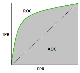
AUC (Area Under The Curve) ROC (Receiver Operating Characteristics) curve also written as AUROC (Area Under the Receiver Operating Characteristics), is a performance measurement for classification problem at various thresholds settings. ROC is a probability curve and AUC represents the degree or measure of separability. It tells how much model is capable of distinguishing between classes. By our example, the higher the AUC, the better the model is at distinguishing between fraudulent transactions and non-fraudulent ones.

The ROC curve is plotted with TPR(Recall) against the FPR where TPR is on y-axis and FPR is on the x-axis.

An excellent model has AUC close to 1 which means it has a good measure of separability. A poor model has AUC close to 0 which means it has the worst measure of separability. In fact, it means it is reciprocating the result. It is predicting 0s as 1s and 1s as 0s. And when AUC is 0.5, it means the model has no class separation capacity whatsoever. see more details here

Log Loss:

Logarithmic loss (related to cross-entropy) measures the performance of a classification model where the prediction input is a probability value between 0 and 1. The goal of our machine learning models is to minimize this value. A perfect model would have a log loss of 0.

Log loss increases as the predicted probability diverges from the actual label. So predicting a probability of .012 when the actual observation label is 1 would be bad and result in a high log loss. There is a more detailed explanation of the justifications and math behind log loss here.

All the explained metrics can be implemented using the sklearn library

• accuracy
• recall and precision
• auc_roc
• log loss

Thanks for reading, If you like this post, a tad of extra motivation will be helpful by giving this post some claps 👏. I am always open for your questions and suggestions. You can share this on Facebook, Twitter, Linkedin, so someone in need might stumble upon this.

PS: This article was first published on my medium

You can reach me at:

LinkedIn: Paul Okewunmi

Twitter: paul_okewunmi

references

• Hands-On Machine Learning with Scikit-Learn and TensorFlow by Aurélien Géron
• Understanding AUC — ROC Curve